Relative Frequency Exploration

6/28/18

Consider flipping a coin for i = 1 to N flips. For trial i, if the coin lands on Heads, write down X_i = 1. If the coin lands on Tails, write down X_i = 0. Do this for all N flips. Next, at each flip i, calculate the relative frequency of Heads as f_i = sum(X_j, j = 1 to i)/i. For example, if the observed results are 0, 1, 1, 1, 0, 1, then f_is are 0, 1/2, 2/3, 3/4, 3/5, and 4/6, respectively.

We intuitively recognize that this relative frequency will "settle down". It might not settle down to a theoretical p = 50%, however, and that is OK. For example, the coin could be biased or the object might not be a coin (it could be a tack for example).

Call the last relative frequency f_N. One question is, how close to p does f_N have to be before you conclude f_N = p? This is both an absurd question and an important question. It is an absurd question, because we know f_N is not p (although it could be by chance). It is an important question because we understand that .5, for example, is for all intents and purposes equal to .499999 or .500001 (and if those don't do it for you, just add more 9s and 0s), much like we use 3.141595 to estimate pi for many important engineering tasks, and this type of frequentist interpretation of probability as a long-term relative frequency is the most dominant and objective.

Consider a tolerance or epsilon, e, and a distance, d = |f_N-p|. We might conclude f_N = p if |f_N-p| < e for some small e>0. For example, if e = .001, and after N trials we find that f_N is in the interval [.499, .501], we conclude f_N = p.

I set to test this out for a coin flip for different e, as well as for a varying number of flips N. I used a "digital coin", the random function in Excel. You can, however, do this exact same thing for a real, physical coin. For each (e, N) combination, I ran 10,000 repetitions. However, I only did 100 repetitions for the (e = .000001, N = 100,000) pair, since it was taking too long on any computer I used due to the computations involved with the N coin flips being refreshed. I kept track of the percent of time f_N landed in the interval. Let's call this percentage P%.

Here are the results:

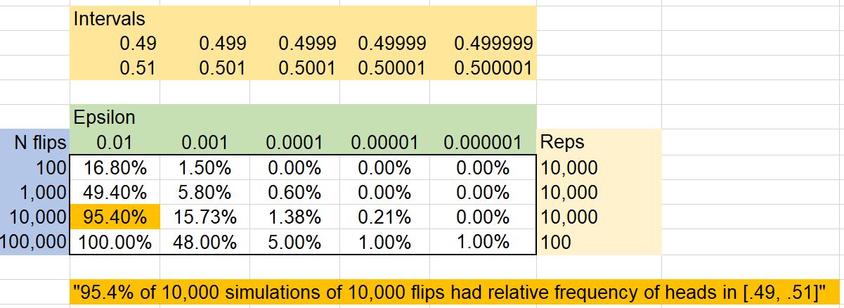
We can see that 95.4% of the 10,000 simulations of 10,000 flips had relative frequency of Heads in [.49, .51]. Also, it is clear that the P% decreased as e decreases. Also, for a fixed e, as N increases the P% gets larger. These results matched my intuition pretty well, as well as what I know about the Strong Law of Large Numbers. However, I was somewhat surprised that the P% got small very fast when I decreased e by an order of magnitude or decreased N by an order of magnitude.

As I mentioned, I did these simulations in Excel. You can download the spreadsheet here. It has a Visual Basic macro you can run by doing Ctrl-J, after you enter the information in the yellow highlighted boxes you want (p, e, and number of simulations).

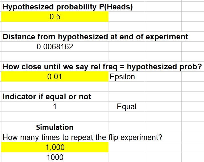
You will also need to fill down the data accordingly for how many flips, N, you want to use.

Thanks for reading.