Multiple Logistic Regression:
Predicting Coronary Heart Disease
A thesis submitted to the Department of
Mathematics of Southern Oregon University in partial fulfillment of the
requirements for the degree of
BACHELOR OF SCIENCE
in
MATHEMATICS
2001
APPROVAL PAGE
To my heroes, the mathematicians and
statisticians of the past and present,
for asking interesting questions for the
mathematicians and statisticians of the future.
ACKNOWLEDGEMENTS
The author wishes to acknowledge Professors
Daniel Kim and Lisa Ciasullo of the Southern Oregon
University Mathematics Department for the assistance they provided. Thanks is also due to the entire Math 490 class, for their
patience and countless suggestions.
ABSTRACT OF THESIS
APPLIED AND THEORETICAL MULTIPLE LOGISTIC
REGRESSION
This thesis addresses the topic of applied
and theoretical multiple logistic regression. Specifically, this study traces
the roots of the logistic regression model, presents a derivation of how the
estimated regression coefficients are obtained, and applies this knowledge to
analyze the Framingham Heart Study data.
Research took three main routes: 1) a
historical overview of the suspected origins of the logistic and logistic
regression model; 2) the derivations of many important features of the logistic
regression model, including how the estimated regression coefficients are
obtained; 3) the application of this information to the Framingham Heart Study
data, and the analysis of the results.
The research shows that the risk of
Coronary Heart Disease (CHD) increases with age, being of the male gender,
having high blood pressure, high cholesterol, and increased smoking of
cigarettes.
VITA
UNDERGRADUATE
SCHOOLS ATTENDED:
Southern
DEGREES
AWARDED:
Bachelor of Science in Mathematics, 2001,
AREAS
OF SPECIAL INTEREST:
Multiple Linear Regression
Hypothesis Testing
Economics
Zheng Manqing style Taijiquan
AWARDS
AND HONORS:
Southern
1999
Southern
Award, 1999
PUBLICATIONS:
"Problem # 688", The
College Mathematics Journal, Vol.
31, No. 5, November, 2000.
TABLE OF CONTENTS
CHAPTER PAGE
I. INTRODUCTION . . . . . . . 1
II. HISTORICAL OVERVIEW AND PRELIMINARIES . . 3
Logistic Model . . . . . . . 4
Regression . . . . . . . 4
III. THE LOGISTIC REGRESSION MODEL . . . . 5
CHD vs. AGE 7
Mean CHD vs. AGE 8
Prediction Model . . . . . 9
Conditional Expectation 9
Link Function 9
Error Term 10
Mean 11
Variance 11
Final Model . . . . . . . 12
IV. ESTIMATING THE REGRESSION COEFFICIENTS . . 13
The
Method of Maximum Likelihood . . . 15
Regression Matrices . . . . . 17
Iteratively Reweighting
Algorithm . . 18
Initial Estimates 19
V. MODEL DIAGNOSTICS . . . . . . 21
Pearson Residual . . . . . 22
Interpretation . . . . . . 23
Conclusion . . . . . . 24
WORKS CITED . . . . . . . . 25
LIST OF TABLES AND FIGURES
PAGE
Table 1. AGE and CHD Status of 100
Subjects . . 6
Table 2. Frequency Table . . . . . 8
Table 3. Descriptions of Variables . . . 13
Table 4. Correlation Matrix . . . . . 14
Table 5. Regression Matrices . . . . . 17
Table 6. Initial Estimates of
Coefficients . . 19
Table 7. Estimated Coefficients . . . . 20
Table 8. Odds of Having CHD . . . . . 23
Figure 1. CHD vs.
AGE . . . . . . 7
Figure 2. Mean
CHD vs. AGE . . . . . 8
Figure 3. Prediction
Model . . . . . 10
Chapter
1: INTRODUCTION
Logistic regression is one of the most
popular and effective ways to analyze data with a binary outcome. This paper
uses logistic regression to develop a model to assess the probability of someone
having coronary heart disease (CHD). A probability of having CHD is obtained
based on the following biological factors: age, gender, systolic blood
pressure, diastolic blood pressure, total serum cholesterol, and number of
cigarettes smoked per day. The data studied is a random sample of 1,000 from
the original Framingham Heart Study, which was started in 1948 in
The function of the coronary arteries is to
supply blood to the heart muscle. Coronary diseases can reduce oxygen intake to
the heart, which may lead to heart attacks or death. Plaque build-up in the
inner lining of an artery is the most common form of coronary disease.
Unfortunately, heart disease is the number
one killer of both men and women in the
Chapter
II: HISTORICAL OVERVIEW AND
PRELIMINARIES
There is no exact data when logistic
regression was introduced. We can, however, logically trace its roots back to
mathematicians in the 18th century who were studying differential
equations. Using the results of differential equations, the economist and
clergyman Thomas Malthus provided people with the
alarming possibility that exponential human growth could threaten the global
environment (de Steiguer 5). For example, any
exponentially growing population sooner or later exceeds the physical and
biological limits of its environment. Thus, the exponential
model, which providing potentially good estimates of population trends, is not
realistic in the long run.
The exponential model overlooked the fact
that every environment has finite space and resources. This inherent quality of
an environment is called a carry capacity. A carrying capacity is the maximum
number that a population can be. As the population increases towards the
carrying capacity, its growth must slow. Therefore, the population's growth
rate is proportional both to the population itself and to the difference
between the carrying capacity and the population (Ostebee
645).
In symbols, we can say that![]() , where
, where![]() represents the population at time
represents the population at time![]() ,
,![]() represents the growth rate of the population at time
represents the growth rate of the population at time![]() ,
,![]() the long-term carrying capacity of the environment, and
the long-term carrying capacity of the environment, and![]() measures the population's reproduction rate.
measures the population's reproduction rate.
Separating variables yields:
![]() .
.
Notice
that:
![]()
We can leave out the absolute-value sign if
we note that![]() .
.
Therefore, solving for![]() is straightforward:
is straightforward:
![]()
![]()
![]()
![]()
![]()
Letting![]()
![]()
To apply this function, we only need to
choose appropriate values for the constants. These constants can be obtained
from past data or estimated by various experiments.
Over time, statisticians realized that they
could use the logistic model with various kinds of data, not just populations
of people and animals. Also, they adapted the regression model to enable it to
handle multiple predictors, which is a more realistic approach. All of these
changes made logistic regression a very powerful and useful regression
technique.
Why would someone want to learn regression
in the first place? If we are studying some phenomenon and collecting data on
it, we will eventually want to be able to say something intelligent about it.
However, data collection can be expensive, time consuming, and in some cases,
impossible to carry out completely. This is where regression analysis comes in.
We would like to find some function that will estimate data that we do not
have, by using the data that we do have. Regression analysis is employed in all
types of sciences (Mendenhall 544) and is an extremely powerful tool.
Chapter
III: THE LOGISTIC REGRESSION MODEL
The transition from the logistic model to
the logistic regression model is probably best illustrated by a concrete
example. However, logistic regression cannot be used with any type of data. The
use logistic regression, the response variable must be polytomous.
That is, the response variable can only take on a finite number of values. Most
commonly, the response variable will only take on two values, in which case the
response variable is called binary or dichotomous. The predictors, however, can
either be continuous or discrete.
Table 1 contains an example of data that is
suitable to be used in logistic regression. The data illustrates a common
situation in the medical field. Note that the response variable CHD can be
regarded as a dichotomous variable by assigning appropriate codes to indicate
the status of CHD. That is, we can assign 1 to CHD if the patient has the disease, and 0 to CHD otherwise.
Table 1 Age and CHD Status of 100 Subjects
|
ID |
AGE |
CHD |
ID |
AGE |
CHD |
ID |
AGE |
CHD |
ID |
AGE |
CHD |
|
1 |
20 |
0 |
26 |
35 |
0 |
51 |
44 |
1 |
76 |
55 |
1 |
|
2 |
23 |
0 |
27 |
35 |
0 |
52 |
44 |
1 |
77 |
56 |
1 |
|
3 |
24 |
0 |
28 |
36 |
0 |
53 |
45 |
0 |
78 |
56 |
1 |
|
4 |
25 |
0 |
29 |
36 |
1 |
54 |
45 |
1 |
79 |
56 |
1 |
|
5 |
25 |
1 |
30 |
36 |
0 |
55 |
46 |
0 |
80 |
57 |
0 |
|
6 |
26 |
0 |
31 |
37 |
0 |
56 |
46 |
1 |
81 |
57 |
0 |
|
7 |
26 |
0 |
32 |
37 |
1 |
57 |
47 |
0 |
82 |
57 |
1 |
|
8 |
28 |
0 |
33 |
37 |
0 |
58 |
47 |
0 |
83 |
57 |
1 |
|
9 |
28 |
0 |
34 |
38 |
0 |
59 |
47 |
1 |
84 |
57 |
1 |
|
10 |
29 |
0 |
35 |
38 |
0 |
60 |
48 |
0 |
85 |
57 |
1 |
|
11 |
30 |
0 |
36 |
39 |
0 |
61 |
48 |
1 |
86 |
58 |
0 |
|
12 |
30 |
0 |
37 |
39 |
1 |
62 |
48 |
1 |
87 |
58 |
1 |
|
13 |
30 |
0 |
38 |
40 |
0 |
63 |
49 |
0 |
88 |
58 |
1 |
|
14 |
30 |
0 |
39 |
40 |
1 |
64 |
49 |
0 |
89 |
59 |
1 |
|
15 |
30 |
0 |
40 |
41 |
0 |
65 |
49 |
1 |
90 |
59 |
1 |
|
16 |
30 |
1 |
41 |
41 |
0 |
66 |
50 |
0 |
91 |
60 |
0 |
|
17 |
32 |
0 |
42 |
42 |
0 |
67 |
50 |
1 |
92 |
60 |
1 |
|
18 |
32 |
0 |
43 |
42 |
0 |
68 |
51 |
0 |
93 |
61 |
1 |
|
19 |
33 |
0 |
44 |
42 |
0 |
69 |
52 |
0 |
94 |
62 |
1 |
|
20 |
33 |
0 |
45 |
42 |
1 |
70 |
52 |
1 |
95 |
62 |
1 |
|
21 |
34 |
0 |
46 |
43 |
0 |
71 |
53 |
1 |
96 |
63 |
1 |
|
22 |
34 |
0 |
47 |
43 |
0 |
72 |
53 |
1 |
97 |
64 |
0 |
|
23 |
34 |
1 |
48 |
43 |
1 |
73 |
54 |
1 |
98 |
64 |
1 |
|
24 |
34 |
0 |
49 |
44 |
0 |
74 |
55 |
0 |
99 |
65 |
1 |
|
25 |
34 |
0 |
50 |
44 |
0 |
75 |
55 |
1 |
100 |
69 |
1 |
(Hosmer 3)
As researches, the doctors would like to know
what can be said about the relationship between the dependent variable CHD and
the predictor variable AGE. The doctors start by constructing a scatterplot of CHD vs AGE.
When analyzing data, especially in a
regression setting, it is important to first create a scatterplot
to roughly assess the relationship between the variables. However, in this case
the dependent variable CHD is discrete, and as Figure 1 shows, a scatterplot is not very useful (Hosmer
2).
Figure 1 CHD vs AGE
Because we essentially have two horizontal bands,
it is clear that it will be near impossible to find a useful function that will
predict CHD given AGE. It does, however, seem that as AGE increases there are
more cases of CHD = 1, but there are several exceptions. In order to find a
more exact relationship between AGE and CHD, we will focus our attention on the
probability of a subject having CHD. To accomplish this, consider the
proportion of individuals who have CHD within a certain AGE interval. Table 2
shows the results.
Table 2 Frequency
Table
|
Age Group |
Midpoint |
% CHD |
|
20-29 |
24.5 |
0.1 |
|
30-34 |
32 |
0.13 |
|
35-39 |
37 |
0.25 |
|
40-44 |
42 |
0.33 |
|
45-49 |
47 |
0.46 |
|
50-54 |
52 |
0.63 |
|
55-59 |
57 |
0.76 |
|
60-69 |
64.5 |
0.8 |
Next, we plot the proportion of individuals
with CHD versus the midpoint of each AGE interval. Doing this produces Figure
2.
Figure 2 %CHD vs Mean
AGE
This scatterplot
provides much more insight into the relationship between CHD and AGE than
Figure 1. However, our goal is to find a functional form to describe this
relationship. In order to do this, we will focus our attention on the
conditional expectation.
Let![]() denote the column vector of all
denote the column vector of all![]() predictors. The proportion of individuals with the
characteristic
predictors. The proportion of individuals with the
characteristic![]() is denoted as
is denoted as![]() . Because these are proportions,
. Because these are proportions,![]() .
.
Keep in mind that there are an infinite
number of functions that are between zero and 1. With hard theoretical work and
empirical motivation, statisticians found a function that works effectively in
many applications (Ryan 256), and has a similar structure to the logistic model
from differential equations.
Let![]() , called the link function, denote a linear combination of
the
, called the link function, denote a linear combination of
the![]() predictors.
predictors.
![]() .
.
It is an interesting question as to why a
linear combination is used instead of some other relation. As it turns out, the
link function has been found to work in many theoretical and applied settings (McCullagh 107), and is what works best in logistic
regression.
The main objective of logistic regression
is to build a model to predict![]() . The prediction model that has been found to work is:
. The prediction model that has been found to work is:
![]() .
.
Graphically, this relationship is shown in
Figure 3.
Figure 3 Prediction Model
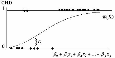
The random variable![]() is called the error, and it expressed an observation's
deviation from the conditional mean. In linear regression, for example, the
common assumption is that
is called the error, and it expressed an observation's
deviation from the conditional mean. In linear regression, for example, the
common assumption is that![]() . However, this is not the case with a binary response
variable. In this situation, we may express the values of the response variable
given
. However, this is not the case with a binary response
variable. In this situation, we may express the values of the response variable
given![]() as:
as:
![]()
Here the quantity![]() may assume one of two possible values. When
may assume one of two possible values. When![]() ,
,![]() with probability
with probability![]() . When
. When![]() ,
,![]() with probability
with probability![]() .
.
Using the above information, we can
calculate the mean and variance of the random variable![]() .
.
The definition of the expected value of a
discrete random variable![]() , with probability distribution function
, with probability distribution function![]() , is defined as:
, is defined as:
![]()
Therefore, the expected value of![]() is found to be:
is found to be:
![]()
![]() .
.
This says that even though some errors may
be large or small, we can expect the mean of them to be zero, which is
reassuring if we expect to have a good model.
Similarly, the variance of a discrete
random variable![]() , with a probability distribution function
, with a probability distribution function![]() , is defined as:
, is defined as:
![]() .
.
Using this information, with the fact that![]() , gives:
, gives:
![]()
![]()
![]() .
.
Because we know the structure of our entire
regression model, we are now able to present the regression model in full:
![]() ,
,
where![]() has mean 0 and variance
has mean 0 and variance![]() .
.
We have the model now, but notice that it
depends on the unknown coefficients. These coefficients cannot just be
'guessed'. The coefficients are parameters that have to be estimated from the
existing data. In the next chapter, we will develop a reliable estimation
process for accomplishing this important task.
Chapter
IV: ESTIMATING THE REGRESSION
COEFFICIENTS
The data that this paper analyzes is a
random sample from the original Framingham Heart Study (Bown,
A-28). There are many variables to consider when trying to
determine what is responsible for CHD. The scientists involved with the
Table 3 Descriptions of Variables
CHD: Coronary heart disease, 1: CHD present, 0: CHD absent
----
GEN: Gender, 1: male, 0: female
AGE: Age (years)
SBP: Systolic blood pressure – when heart is pumping (mm Hg)
(Mercury)
DBP: Diastolic blood pressure – when heart is at rest (mm Hg)
CHL: Total serum cholesterol level (mg/dL)
CIG: Cigarettes smoked (#/day)
To illustrate the relationships between the
six predictors, a correlation matrix is shown in Table 4.
Table 4 Correlation Matrix
|
|
GEN |
AGE |
SBP |
DBP |
CHL |
CIG |
|
GEN |
1 |
|
|
|
|
|
|
AGE |
-.0310 |
1 |
|
|
|
|
|
SBP |
.0108 |
.3532 |
1 |
|
|
|
|
DBP |
.1279 |
.2298 |
.7930 |
1 |
|
|
|
CHL |
-.0307 |
.2877 |
.2119 |
.1597 |
1 |
|
|
CIG |
.3632 |
-.1525 |
-.0423 |
-.0281 |
.0436 |
1 |
As Table 4 shows, it appears that there is
high correlation only associated with DBP and SBP. There also seems to be
moderate correlation between SBP and AGE, and CIG and GEN.
Before we can use logistic regression to
analyze this data, we must ask if these predictors are any good. That is, do
our predictors do a good job of distinguishing who has CHD? If so, the we expect the population means of the predictors for
each group CHD = 1 and CHD = 0 to be different. Using the technique of
multivariate analysis of variance (MANOVA), we can shed some light on the
answer to this question.
The hypotheses we are concerned with are:
 vs.
vs. 
The idea of MANOVA relies on the F-test.
The actual form of the test statistics (Johnson 224) yields a p-value which is
less than .001. We therefore reject![]() at the 5% level of significance, and conclude that the
population means are, in fact, different.
at the 5% level of significance, and conclude that the
population means are, in fact, different.
The next step is to actually estimate the
regression coefficients. The most common technique statisticians are familiar
with is the method of least squares. However, the method of least squares fails
in the case of logistic regression because the necessary assumptions are
violated. In logistic regression, the method of maximum likelihood is used to
estimate the coefficients.
The sample likelihood function is defined
as the joint probability function of the![]() random variables, which constitute the sample. Specifically,
for a sample size
random variables, which constitute the sample. Specifically,
for a sample size![]() the corresponding random variables are:
the corresponding random variables are:

In most cases, it is reasonable to assume
that the![]() ,
,![]() are independent. By the multiplicative law for independent
events, the joint probability function is then:
are independent. By the multiplicative law for independent
events, the joint probability function is then:
![]()
In words, the likelihood function gives the
probability of observing a sequence of 0's and 1's, which corresponding to
people having CHD or not. It should be noted that the assumption of independent
Bernoulli random variables might not always be plausible,
however, for the most part we are safe with that assumption (Ryan 258).
Maximum likelihood estimates are usually
obtained by maximizing the logarithm of the likelihood function, especially
when the likelihood function is complicated. This is acceptable to do because
the likelihood function and the logarithm of the likelihood function both
achieve their maximums at the same place, because the logarithm function is
monotonic. This also has the added bonus of making the calculus involved more
tractable.
Taking the logarithm of each side of the
likelihood equation produces:
![]()
 .
.
To find our maximum likelihood estimates of![]() , we want to set all the partial derivates of
, we want to set all the partial derivates of![]() equal to zero, and solve the resulting non-linear system
simultaneously for the
equal to zero, and solve the resulting non-linear system
simultaneously for the![]() . Because this is a non-linear system of equations, solving
the system requires an approximation method. One of the most popular methods is
the iteratively reweighting algorithm, which relies
on
. Because this is a non-linear system of equations, solving
the system requires an approximation method. One of the most popular methods is
the iteratively reweighting algorithm, which relies
on
Introducing matrix notation will aid us in
this process. Table 5 details the matrices involved with estimating the
coefficients in logistic regression.
Table 5 Regression Matrices


The likelihood equations that we obtain
from differentiating![]() are:
are:
![]() , and
, and
![]() , for
, for![]()
More concisely, we can write all of the![]() likelihood equations using matrix notation as:
likelihood equations using matrix notation as:
![]() .
.
To use the iteratively reweighting
algorithm, we must use the idea of ![]() . This is equivalent to computing
. This is equivalent to computing![]() , which equals
, which equals![]() .
.
From its definition, we can compute![]() and
and![]() . Therefore,
. Therefore, ![]() , so
, so![]()
![]() .
.
Now that we have all the necessary parts
that
![]()
where![]() is the iteration number.
is the iteration number.
Solving this for![]() yields:
yields:
![]()
This algorithm is dependent on![]() . The method for initially estimating these coefficients is
shown in Table 6 (Hosmer 35).
. The method for initially estimating these coefficients is
shown in Table 6 (Hosmer 35).
Table 6 Initial Estimates of Coefficients

![]()
Where![]() and
and![]() , and
, and

After this algorithm is carried out, we
have our fitted model. Using the statistics software program S+ 2000, the
coefficients, shown in Table 7, were estimated.
Table 7 Estimated Coefficients

Therefore
our fitted model is:
![]()
It is tempting to want to substitute in an
age, blood pressure, and so on, in order to estimate someone's probability of
having CHD. However, we must know whether or not this fitted model is good
before we can use it.
Chapter V: MODEL DIAGNOSTICS
The last chapter presented a method for
estimating the coefficients involved in logistic regression. However, does
going through that process guarantee that we have a good fitted mode? The
answer is a surprising "No". Also, what does it mean to have a "good" model?
The branch of regression that attempts to answer these questions is called
model diagnostics.
The main focus of model diagnostics is on
the concept of goodness of fit. There are many ways to measure goodness of fit.
Some of the ways are through analysis of the likelihood ratios, deviance
residuals, various forms of![]() , and through the Pearson residuals. This chapter focuses on
the Pearson residuals because of their straightforward interpretations.
, and through the Pearson residuals. This chapter focuses on
the Pearson residuals because of their straightforward interpretations.
In order to build these residuals, let![]() denote the number of subjects with the same covariate pattern
denote the number of subjects with the same covariate pattern![]() . Note that
. Note that![]() .
.
Let![]() denote the number of positive responses,
denote the number of positive responses,![]() , among the
, among the![]() subjects with
subjects with![]() . Note that
. Note that![]() , the total number of subjects with
, the total number of subjects with![]() .
.
We can now say that the expected number of
positive response is:
![]()
The Pearson residual is defined and denoted
as:
 ,
,
and the summary statistic based on these results is:
 ,
,
where![]() denotes the number of distinct values of
denotes the number of distinct values of![]() observed.
observed.
Once again we set up two hypotheses:
![]() The model does fit the data
The model does fit the data
vs.
![]() The model does not fit the data
The model does not fit the data
This goodness of fit test relies on a![]() distribution with
distribution with![]() degrees of freedom. For the
degrees of freedom. For the ![]() . This is less than the theoretical
. This is less than the theoretical![]() . Therefore, we fail to reject
. Therefore, we fail to reject![]() at the 5% level of significance, and conclude that there is
evidence of our model fitting the data well.
at the 5% level of significance, and conclude that there is
evidence of our model fitting the data well.
One way to interpret the model is through
the estimated coefficients. In linear regression, the interpretation is
straightforward. In logistic regression we are working with a non-linear
function, and therefore our interpretation must change accordingly.
In the
Specifically, we are interested in![]() . One can work out, from the definition of odds, that
. One can work out, from the definition of odds, that![]() , which is equivalent to:
, which is equivalent to:
![]() =
=
![]()
Using these results we can assess the odds
of having CHD, ceteris paribus. This was done with all of the predictors, and
the results are summarizes in Table 8.
Table 8 Odds of Having CHD
|
Predictor |
Unit Change |
Odds Change |
|
GEN |
1 |
2.75 |
|
AGE |
10 years |
2 |
|
SBP |
15 mm |
1.3 |
|
DBP |
15 mm |
.97 |
|
CHL |
20 mg |
1.15 |
|
CIG |
5 |
1.06 |
We can see that the unit changes in the
majority of the predictors cause a multiplicative increase in the odds of
having CHD. Particularly disturbing is the impact that being male has on the
odds, and also the relationship that age has with having CHD.
It is interesting to, and somewhat
confusing at first, to see that increases in SBP increase the odds of having
CHD, while increases in DBP lower the odds of having CHD. This apparent anomaly
may simply be the result of analyzing a random sample. It could also be related
with the fact that SBP and DBP have a very large degree of correlation.
Logistic regression is a very powerful tool
in the sciences. It has its roots in calculus and differential equations, and
has been added to and modernized by statisticians to make it what it is today.
By using logistic regression on a random
sample of the original
A more sophisticated study would possibly
include some different variables and include some others. Also, attention needs
to be paid to possible confounding factors, some of which could be exercise,
diet, lifestyle, stress levels, and other biological factors, such as genetics.
There are numerous applications of logistic
regression, and most are contained in the sciences. Logistic regression has
been successfully used for environmental modeling, remote sensing, and disease
classification, just to name a few. With some work, logistic regression can be
extended to handing multiple responses, which would allow for more realistic
situations, such as a disease with multiple stages.
WORKS CITED
Bown, Fred, and Chase,
De
Steiguer, J.E. Age
of Environmentalism.
Hosmer, David W., and Lemeshow, Stanley. Applied
Logistic Regression.
Johnson, Richard A., and Wichern,
Dean W. Applied Multivariate Statistical
Analysis.
McCullagh, P., and Nelder,
J.A. Generalized Linear Models.
Mendenhall, William, and Schaeffer, Richard
L., and Wackerly, Dennis D. Mathematical Statistics with Applications.
Ostebee, Arnold, and Zorn, Paul. Calculus- From Graphical, Numerical, and Symbolic Points of View.
Ryan, Thomas P. Modern Regression Methods.